Most people reach for optical satellite imagery first, and for most questions that’s right. It’s interpretable, familiar, and abundant. It also fails in a specific and inconvenient way: cloud, fog, and smoke put gaps in the record precisely when something interesting is happening, and varying illumination means two dates aren’t cleanly comparable even when both are clear.
Radar has neither problem. Sentinel-1 acquires regardless of weather or daylight, on a repeat cycle, and the archive is open. The catch is that SAR isn’t a photograph — it measures surface roughness and geometry, and it arrives buried in speckle. Getting signal out takes work before analysis starts, and that barrier is why SAR gets left out of projects that would benefit from it.
These are notes from two problems we worked on in 2023, both about water, with deliberately opposite processing pipelines.
Why water is the easy case for radar
Calm water is smooth relative to the radar wavelength. It reflects the signal away from the sensor and returns almost nothing. Land is rough and scatters energy back in all directions, including toward the sensor.
The result is that water appears dark against bright terrain, with a large separation between the two. You don’t need a model to see water in SAR — you need a threshold. That makes water extent one of the most tractable things radar measures, and it’s why both problems below were realistic targets rather than research projects.
Problem one: measuring surface pollution coverage on open water
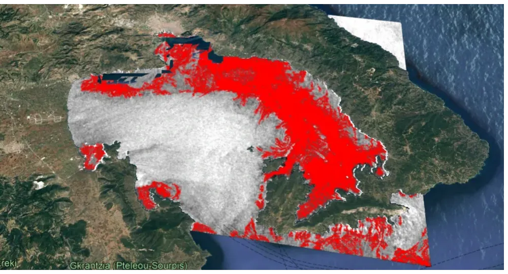
The question. Repeated flooding and drought around Volos pushed freshwater fish into the saltwater of the Pagasetic Gulf, where they died in large numbers. What proportion of the water surface was covered, and how was that changing?
Why radar. Coverage measured on different dates has to be comparable, or the time series is meaningless. Optical imagery couldn’t guarantee that; radar could.
Preprocessing. Crop to the area of interest — delivered scenes cover far wider swaths than needed. Calibrate to sigma0 backscatter, turning sensor digital numbers into a physical quantity comparable across acquisitions. Everything downstream depends on this step; without it there is no time series.
Two decisions worth explaining:
No multilooking. The standard next step averages adjacent pixels, reducing speckle and processing load at the cost of resolution. We skipped it. The task requires distinguishing adjacent surface regions, and a dedicated despeckling stage was coming — so multilooking would have traded away resolution to partly solve a problem being solved properly downstream.
Ellipsoid rather than terrain correction. Terrain correction uses a DEM to compensate for topographic distortion. The area of interest is open water. There is no topography to correct, so a DEM adds cost and nothing else.
Then a land-sea mask, removing the coastline before anything else runs. This is a false-positive strategy more than a preprocessing step — coastal structures never reach the model, so they can’t be misclassified and don’t need filtering afterward.
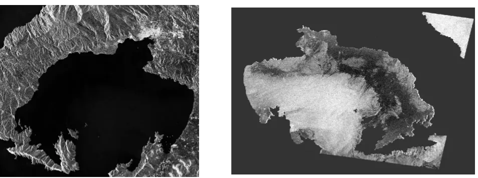
Despeckling. Scenes exported from SNAP into Python via pyroSAR and rasterio, reading VV and VH amplitude bands.
Speckle is the real obstacle to running segmentation on radar. It’s multiplicative interference noise, not sensor noise, so conventional denoising treats it wrongly, and filters that do suppress it do so by smoothing away the fine structure segmentation needs. SAR2SAR is a learned despeckler that removes speckle while preserving low-level detail at full resolution — which is what makes the next step viable at all.
Segmentation. A fine-tuned MIDLN model produces per-detection masks and confidence scores; detections above an experimentally determined threshold are composited and converted into coverage as a percentage of open water in the scene.
**Status.**Delivered and Still Running, Monitoring Changes to Nearby Areas
Problem two: flood and water-level change across farmland
The question. A prospective client wanted to understand vacant and agricultural land — nearby activity, changes in water sources and reservoirs, land hydration across the year, and evidence of flooding or runoff.
Why we did it. This was internal. The proposal would either commit to radar processing or it wouldn’t, and committing to a capability you haven’t tested is how a project goes wrong six months in. A few days of work turned the question into an answer before it turned into a promise.
Preprocessing, inverted. Sentinel-1 scenes across as much of a year as available, June as baseline. Crop, then multilook — here the resolution cost is irrelevant, since the target is regional water extent, and the speed gain is real. Calibrate to sigma0. Terrain correct, because this is land and topographic distortion matters, even where much of the area is flat.
Then a step the Gulf work didn’t need: backscatter distributions were badly skewed, most pixels very low with a long thin tail, leaving images near-black. Converting linear values to decibels produced interpretable imagery and a histogram that could be stretched to bring out the regions of interest.
Change detection without a model. Two processed timesteps, registered by geolocation, composited into RGB: baseline intensity into red, test date into green and blue.
| Appearance | Interpretation |
|---|---|
| Strong red | Water in the test date, land in the baseline — newly flooded |
| Strong blue/green | Water in the baseline, land in the test date — dried or receded |
| Uniformly dark | Low backscatter in both — permanent water |
| Light, even tone | Similar response — no significant change |
No training, no labels, no model. The physics does the work, and the output is directly readable by someone who has had the colour convention explained to them once.
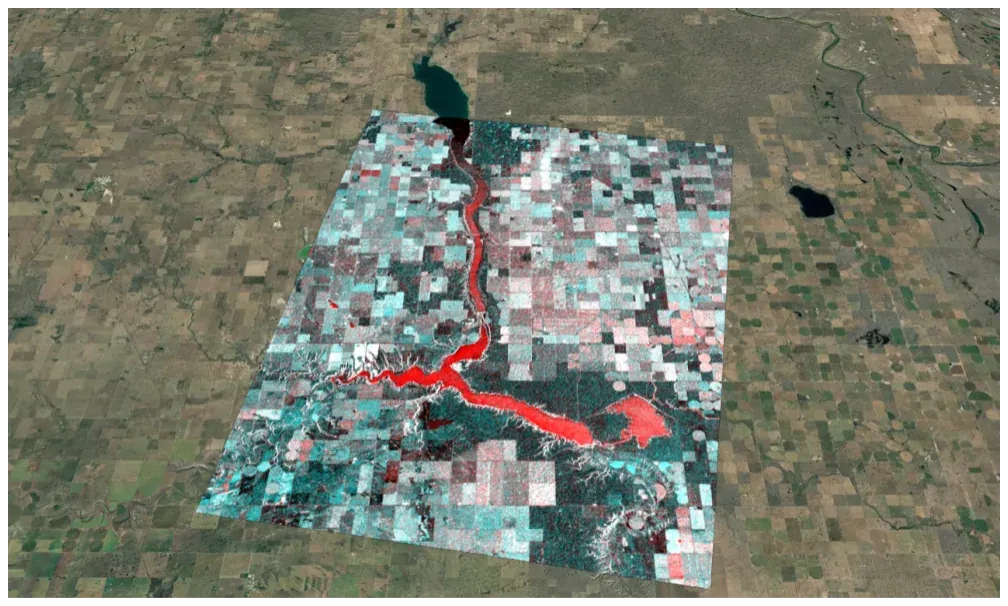
Status. Internal assessment. It answered its question — seasonal water change is extractable from radar at acceptable processing cost — and radar processing went into the proposal on that basis.
The general point
The two pipelines share a data source and a toolbox and agree on almost nothing else.
| Pollution coverage | Flood detection | |
|---|---|---|
| Multilooking | Skipped — detail needed | Applied — regional extent only |
| Geometric correction | Ellipsoid — no terrain to correct | Terrain — land, distortion matters |
| Land-sea mask | Applied | Not applicable |
| Despeckling | SAR2SAR before segmentation | Not needed at this resolution |
| Method | Learned segmentation | Physics-based change composite |
| Output | Coverage percentage | Interpretable change image |
Run the Gulf pipeline on the flood problem and you spend compute preserving detail nobody needs. Run the flood pipeline on the Gulf and multilooking destroys the resolution the segmentation depends on, before it starts.
There is no default SAR pipeline. There are a dozen or so decisions, each of which has a right answer only once you know what’s being measured — which is most of what “SAR is hard to work with” actually means. It isn’t that the data is difficult. It’s that the processing isn’t separable from the question.
Limits worth stating
- Radar sees roughness and geometry, not identity. It distinguishes surface matter from open water; it doesn’t tell you what the matter is.
- Change detection shows change, not cause. Flooding, irrigation, seasonal variation, and reservoir management all look similar without context.
- Resolution sets a floor. The minimum size of a land-based feature or object that can be reliably detected and resolved is 20 to 22 metres
- Segmentation thresholds encode a preference, not an objective standard. Where the threshold sits is a decision about false positives versus misses, and it belongs to whoever bears the cost of each.
If this is relevant to you
Both problems came down to the same thing: a measurement that had to mean the same thing on every date, in conditions where optical imagery couldn’t guarantee that. If you have a monitoring question shaped like that, radar is probably worth testing — and testing is cheap relative to building on an assumption.