A European electricity distribution utility had five years of meter readings, service records, and inspection outcomes, and no systematic way to decide which accounts its technicians should inspect for power theft. Inspections were effectively unprioritized, and the hit rate showed it: 0.4% of inspected accounts turned out to be stealing power.
We built a model that scores accounts by likelihood of theft, along with explanations of what drove each score. In the first inspection cycle run against the scores, the hit rate rose to just under 3% — 7.5× more theft found for the same inspection effort.
Then we handed the whole thing to their data science team, environment and all, so they could retrain and extend it without us.
The problem
Power theft — meter tampering, unmetered connections, manipulated readings — is a persistent revenue loss for distribution utilities, and the only way to confirm it is to send a technician to the site. Inspection capacity is therefore the binding constraint, and every inspection of a legitimate account is capacity spent finding nothing.
Without prioritization, the utility’s inspections were finding theft 0.4% of the time. Nearly all inspection effort produced no result.
The utility had the raw material to do better: five years of accumulated meter readings, service request and completion records, registration and utility account data, and — critically — the outcomes of investigations they had already performed. That last piece is what made supervised learning possible at all, since it supplies the labels.
The goal was not to detect theft. It was to rank accounts so that technicians reached the right doors sooner.
What we built
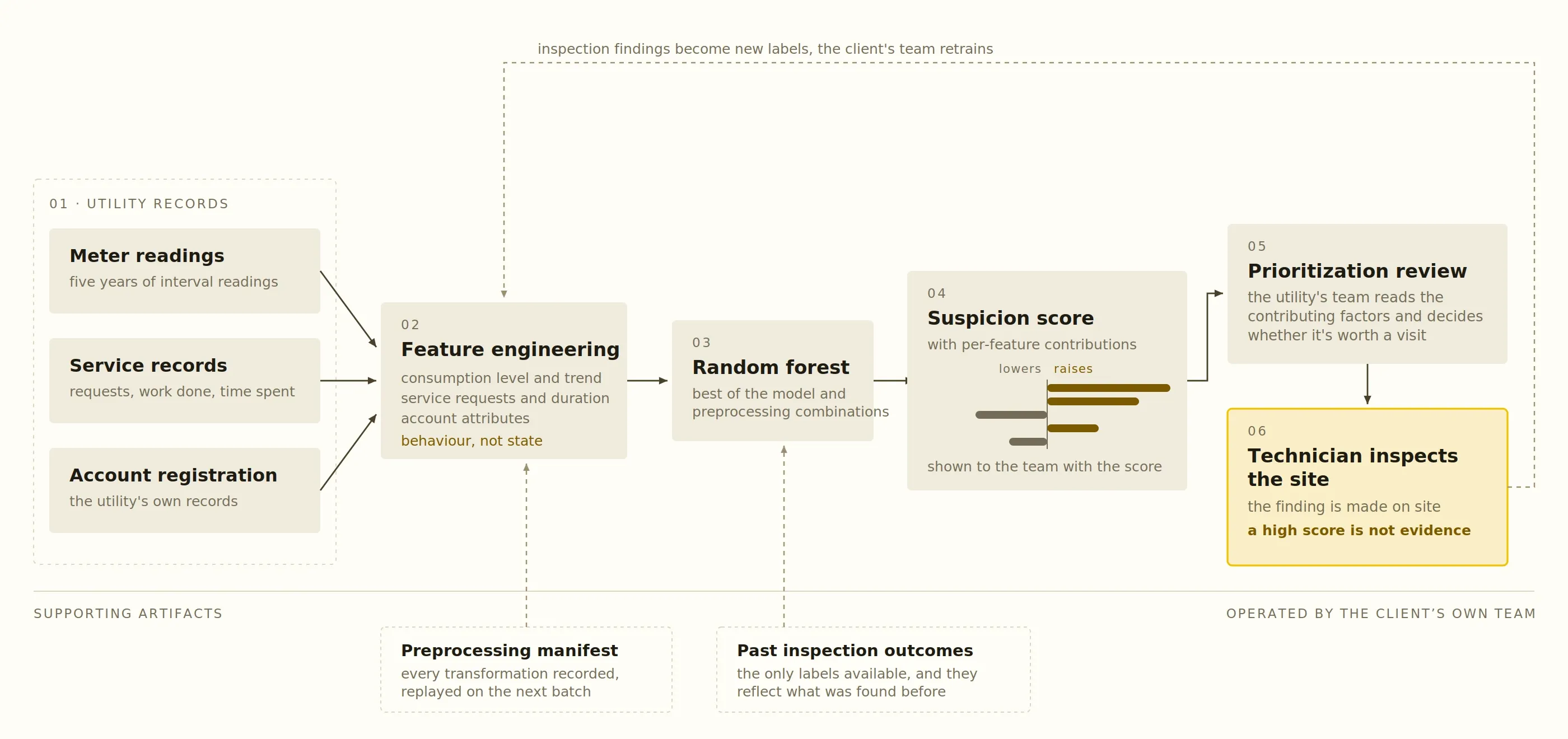
Turning utility records into features
The signal isn’t in any single reading; it’s in patterns across time and across record types. Categorical fields were normalized into one-hot and multi-hot vectors, and the numerical and time series data transformed into features that describe behaviour rather than state:
- Consumption patterns — average power utilization per account across time periods, and whether consumption was trending up or down
- Service interaction — average number and type of service requests per period, and how long technicians spent on them
- Account and registration attributes from the utility’s own records
Labels came from the outcomes of past investigations: did the inspection find theft or not.
An experiment system, not just a model
Most of the engineering effort went somewhere that doesn’t show up in a model card. We built the work as four Jupyter notebooks that chain into a reproducible pipeline:
- Feature generation — runs selected subsets of the feature creation and augmentation functions, so the composition of the dataset itself becomes an experimental variable rather than a fixed assumption.
- Training data preparation — selects the training subset and runs preprocessing, writing out a Parquet file of prepared data plus a manifest recording exactly which transformations were applied.
- Test data preparation — reads that manifest and applies the identical transformations to the test data, so field distributions and one-hot/multi-hot encodings match by construction.
- Training and evaluation — model parameters defined at the top, training and evaluation run below, final metrics out. It also runs a new test set against a previously trained model, provided the same preprocessing manifest was used.
The manifest in step 2 is the important part. Train/test mismatch in encoded categorical features is one of the most common and least visible ways a model that validates well fails in production — a category present in training but absent in the test data silently shifts the vector layout, and nothing errors. Making the transformation record an artifact that step 3 consumes removes the failure mode structurally rather than by discipline.
The model
We compared preprocessing and model combinations across that harness. A random forest performed best, and that’s what shipped.
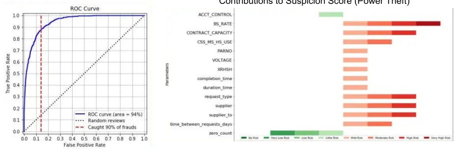
Alongside the suspicion score, the system returns explainability measures — which pieces of information pushed the score up and which pulled it down. This was not a compliance add-on. It’s what lets the utility’s team look at an account, understand why it surfaced, and decide whether it’s worth a visit.
Handing it over
The deliverable was not a scoring endpoint. Using the notebooks, requirement files, and supporting Python scripts, we replicated our development environment on the client’s own servers and trained their data science team to operate it: how to take new customer records, preprocess them consistently, and produce a suspicion score.
More usefully, the same notebooks let them train new models on different datasets, experiment with new feature creation steps, and try different model types as their needs change. The system they received was the one we developed in, not a stripped-down runtime.
This is a deliberate position on how these engagements should end. A utility with five years of proprietary data and an in-house data science team should not need to call a contractor every time the network or the fraud patterns change.
Where the human stays in the loop
The model produces a ranked list and an explanation. It does not determine that anyone is stealing power, and it has no mechanism to act on an account.
Technicians inspect the site and make the finding. Before that, the utility’s teams review the contributing factors behind each score to decide whether an account is worth prioritizing at all. The score changes the order of the queue; it doesn’t shorten the process or substitute for the visit.
That distinction matters more than usual here, because the accusation is serious and the consequences for a wrongly flagged customer are real.
Results
Delivered on time and within budget, operational in the client’s environment by May 2024 in time for the Summer 2024 inspection cycle.
| Unprioritized inspection | Model-prioritized | |
|---|---|---|
| Accounts inspected | 6,000 | 6,000 |
| Theft found | 0.4% (~24 accounts) | just under 3% (~180 accounts) |
Same inspection capacity, 7.5× the theft detected.
At a mean loss of €80 per account per month, the additional accounts identified represent roughly €12,000 per month in recovered revenue from that first 6,000-account cycle — and that recovery continues for as long as those connections would otherwise have remained undetected.
What it doesn’t do
- It doesn’t determine theft. It ranks accounts for inspection. A technician on site makes the finding.
- A high score is not evidence. It reflects statistical similarity to previously confirmed cases and is a reason to look, nothing more.
- Labels come from inspections that were already performed, and those weren’t randomly selected. The model learns from the theft the utility historically found, which may not represent all the theft that exists. We work with the client to expand the amount of inspection performed to catch cases they normal would not review and find
- It’s specific to this utility’s data. Another network would need its own history, its own features, and its own retraining.
- It requires ongoing retraining. Theft patterns shift, particularly once inspections become better targeted — which is exactly why the client operates the training pipeline themselves.
Stack
A random forest in scikit-learn as the production model, developed in a four-notebook Jupyter pipeline with pandas and NumPy over Parquet intermediates and manifest-driven preprocessing consistency. SHAP values accompany each score, so an inspector sees why a meter was ranked where it was rather than a bare number. The environment was replicated on client infrastructure via requirements files and supporting scripts, which is what made the handover possible.